
Detecting change isn’t as straightforward as it sounds
When working with Ecological Momentary Assessment (EMA) data, researchers are often interested in whether psychological processes change over time. Do relationships between variables stay constant, or do they evolve? Time-Varying VAR (TV-VAR) are types of models that are designed to answer exactly that. But detecting change in these models isn’t automatic. You need a way to determine whether apparent variation is real or just noise.
This is where a bootstrap test can be a useful guide.
The core problem: what counts as “real” change?
TV-VAR models estimate parameters, such as means or relationships between variables, as functions of time. If a parameter fluctuates, the model might interpret this as evidence of non-stationarity* in the underlying stochastic process. But detecting fluctuations can also arise purely by chance, especially in shorter time series.
So the key question becomes how we know whether observed variation is meaningful.
Standard statistical tests aren’t always available. For example, in the GAM-based TV-VAR model, p-values for time-varying parameters do not come built in. That makes it difficult to formally test whether a parameter truly changes over time.
Bootstrapping
To solve this, I simulated whether a bootstrapping significance test can be informative in detecting non-stationarity in the underlying process.
Here is how the test works in practice:
- Fit a standard stationary VAR model to the observed time series.
This assumes that, under the null hypothesis, nothing changes over time. - Simulate many new datasets, say 1000, using the estimated parameters. These datasets are guaranteed to be stationary.
- Fit the TV-VAR model to each simulated dataset and calculate the standard deviation across the parameters over time. This gives a distribution of how much variation you would expect purely by chance.
- Fit a TV-VAR model to the real data and also calculate the standard deviation across the parameters. If the found standard deviation is unusually large compared to the bootstrap samples (stationary distribution), it is taken as evidence for real time variation. This can even be quantified in a p-value.
What the results actually show
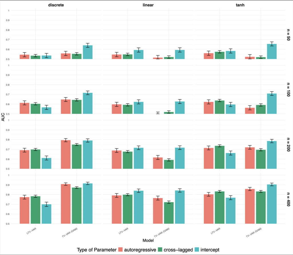
The main takeaway from the results is straightforward. Detecting non-stationarity depends heavily on how much data you have. With 50 time points, both the linear TV-VAR and TV-VAR (GAM) models perform close to chance. Even at 100 time points, their ability to detect change is still limited. Only around 200 time points do both models start to reliably pick up non-stationarity, with strong performance at 400 time points.
There are also clear differences between the models. The LTV-VAR model works best for linear changes in parameters, since it assumes a linear trend over time. In contrast, the TV-VAR (GAM) model performs better for non-linear or abrupt changes, including discrete shifts. For smooth non-linear patterns, both models perform similarly.
Another pattern is that some parameters are easier to evaluate than others. The TV-VAR (GAM) model tends to detect changes in intercepts earlier, while both models need more data to reliably detect changes in autoregressive and cross-lagged effects.
The plot shows how well the two models, LTV-VAR and TV-VAR (GAM), detect non-stationarity across different time series lengths (n = 100, 200, 400) with various parameter changes (discrete, linear, tanh), and parameter types (autoregressive, cross-lagged, intercept), using AUC as the performance metric.
Leave a Reply