Clustering is a popular (unsupervised) technique in data science, widely used for discovering hidden patterns in data without having prior understanding of what such patterns might look like. Examples could be:
- Supply Chain Optimisation – Using clustering to group delivery locations and streamline logistics, reducing cost and enhancing efficiency.
- Customer Segmentation – Clustering helps businesses to group customers based on behaviour, demographics, or purchasing patterns.
While popular methods like K-means and Agglomerative Hierarchical Clustering (AHC) are commonly applied, they often struggle with complex datasets, failing to capture irregular cluster shapes, varying densities, or noisy data.
In this post, we explore advanced clustering algorithms such as, HDBSCAN, Gaussian Mixture Models (GMM), and OPTICS, demonstrating why they often outperform traditional approaches.
*This post is intended for readers with a basic understanding of how each algorithm works.
					library(clValid)
library(tidyr)
library(opticskxi)
library(fpc)
library(mclust)
library(dbscan)
library(ggplot2)
library(cluster)
library(farff)
library(factoextra)

#Load dataset we will use for remainder of the post
data('DS3')
data <- DS3

#dissimilarity_matrix is necessary for several clusteirng algorithms and cluster validation
dissimilarity_matrix <- dist(data)
indices <- data.frame(method = c('K-MEANS', 'HAC', 'GMM', 'HDBSCAN', 'OPTICS'))

# Function for later use to ensure only noise points (cluster 0) are black
plot_clusters <- function(data, clusters, title) {
  unique_clusters <- sort(unique(clusters))

  # Assign colors ensuring noise (0) is black
  colors <- rep("black", length(unique_clusters))  # Default black for noise
  valid_clusters <- unique_clusters[unique_clusters != 0]  # Exclude noise

  # Assign distinct colors only for valid clusters
  if (length(valid_clusters) > 0) {
    colors[unique_clusters != 0] <- rainbow(length(valid_clusters))
  }

  # Map cluster labels to colors
  cluster_colors <- colors[match(clusters, unique_clusters)]

  plot(data, col = cluster_colors, main = title, pch = 20, cex = 1.5,
       xlab = "", ylab = "", xaxt = "n", yaxt = "n")
}
plot(data, pch = 20, main = "Dataset Visualization")
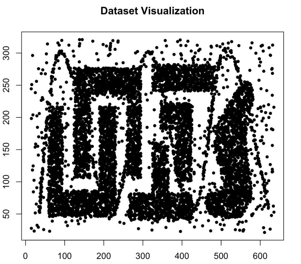
This is the dataset we will analyze. While it is somewhat artificially constructed and unlikely to resemble real-world data exactly, it includes irregular cluster shapes and significant noise, both of which are common in real-world datasets. This makes it an excellent benchmark for evaluating the performance of different clustering algorithms. Normally, data should always be scaled first.
K-Means Clustering
K-means is arguably the most popular clustering algorithm. It partitions the data into k-clusters by assigning each point to the nearest centroid and iteratively updating the centroids to minimise variance within clusters.
Advantages
- Very fast and efficient algorithm, scales well with big data
Disadvantages
- Only performs well for separated, spherical clusters of the same radius and size (Broderick, 2020)
- Random centroid initialisation in first iteration results in highly variable outcomes. K-means++ might by a solution (Rukmi, 2017) by initialising centroids more intelligently.
- Cannot identify noise points
- K-Means performs well when the number of clusters is known in advance. Otherwise, determining the optimal number relies on unreliable methods
Throughout this post, I conduct the analyses as if I had not yet seen the cluster structure. This approach reflects a real-world scenario —especially when dealing with more than three dimensions where it becomes impossible to visually inspect the data.
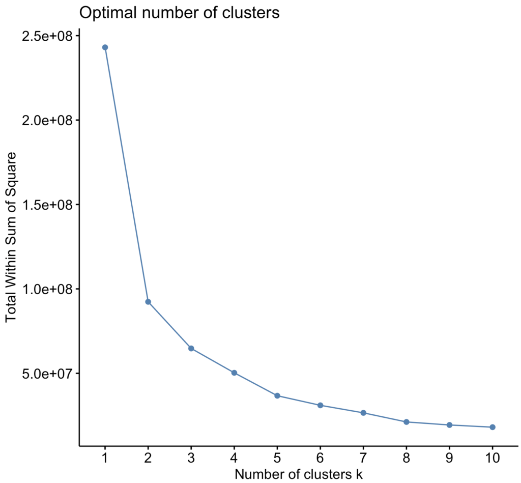
Below I used the ‘Elbow Method‘, wherein you pick a number K that corresponds to where the line in the curve stops decreasing so sharply (Syakur, 2018), i.e., where the within cluster sum of squares isn’t decreasing as sharply anymore. In this case that is 2.
					#Apply the elow method
fviz_nbclust(data, FUN = kmeans, method = "wss")
cluster_kmeans <- kmeans(data, centers = 2, nstart = 20)$cluster
plot_clusters(data, cluster_kmeans, "K-Means Clustering")
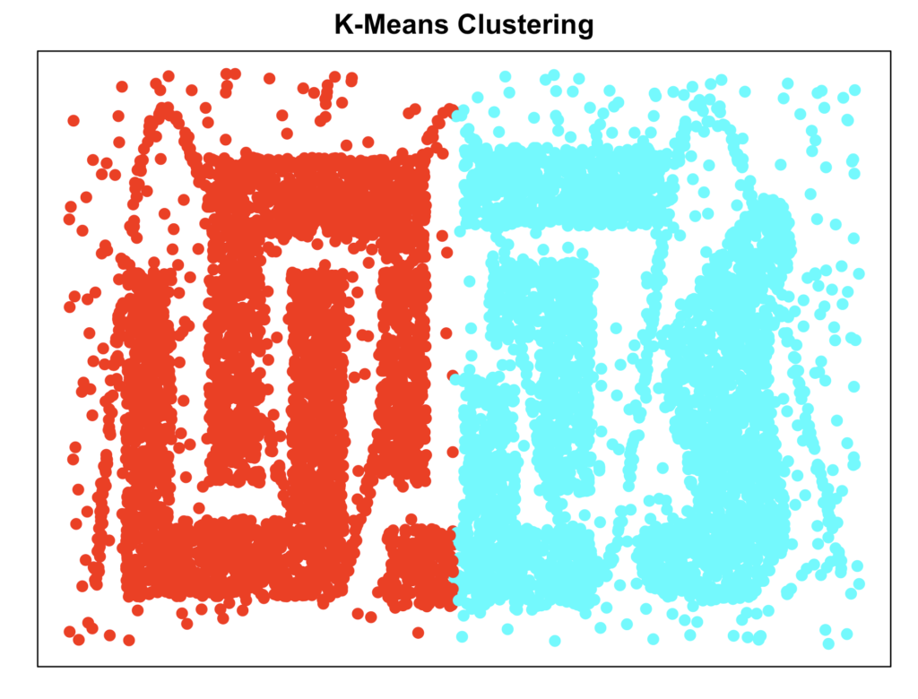
As expected, K-means is largely underfitting the data
Agglomerative Hierarchical Clustering
Agglomerative Hierarchical Clustering is a widely used clustering algorithm that builds a hierarchy of clusters by iteratively merging the closest pairs of clusters until only one remains. It does not require specifying the number of clusters in advance and produces a dendrogram, which can be used to determine the optimal cluster structure.
Advantages
- Does not require to specify number of clusters beforehand
- Can handle non-spherical cluster shapes
- Is able to handle various distance metrics, i.e., ‘singe-linkage‘, ‘complete-linkage‘, etc. Each has their own advantage, see –Adams COS321: Elements of Machine Learning– for an excellent overview.
Disadvantages
- Computationally very expensive, with each iteration it calculates a new dissimilarity matrix
- The dendrogram becomes virtually impossible to properly interpret with large datasets
- Cannot identify noise points
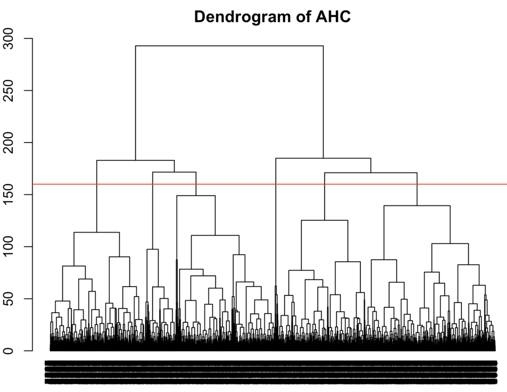
I computed the dendrogram for the ‘average-linkage‘ method. The most optimal number of clusters seem to be 6 since the upward distance is relatively large and it’s not likely to be an underfit. Although something can be said for picking 2
					hclust_result <- hclust(dissimilarity_matrix, method = 'average')
plot(hclust_result, main = "Dendrogram of AHC",
     sub = "", hang = -1, cex = 0.8)
abline(h = 160, col = 'red')
cluster_hclust <- cutree(hclust_result, k = 6)
plot_clusters(data, cluster_hclust, "HAC Clustering")
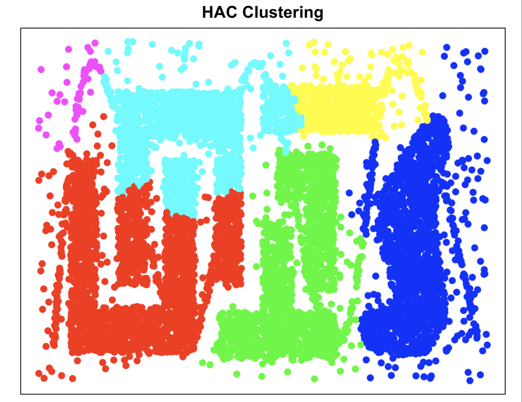
Agglomerative Hierarchical Clustering performs relatively poor, probably because the patterns are too complex.
Gaussian Mixture Models
Gaussian Mixture Models (GGM) is a widely used clustering algorithm that models data as a mixture of multiple Gaussian distributions. Because it initialises various covariance matrices with different shapes and sizes, it allows for more flexibility in capturing complex cluster shapes. The number of clusters can be determined by statistical criteria such as the Bayesian Information Criterion (BIC) or Akaike Information Criterion (AIC)
Advantages
- Could potentially handle noise points by assigning low probabilities to those points
- Can handle non-spherical cluster shapes of different sizes
Disadvantages
- Computationally expensive
- Sensitive to violations of normally distributed data, so cannot handle very complex cluster shapes
The Mclust() function determines the optimal number of clusters based on the BIC by default
					cluster_gmm <- Mclust(data)$classification
plot_clusters(data, cluster_gmm, "GMM Clustering")
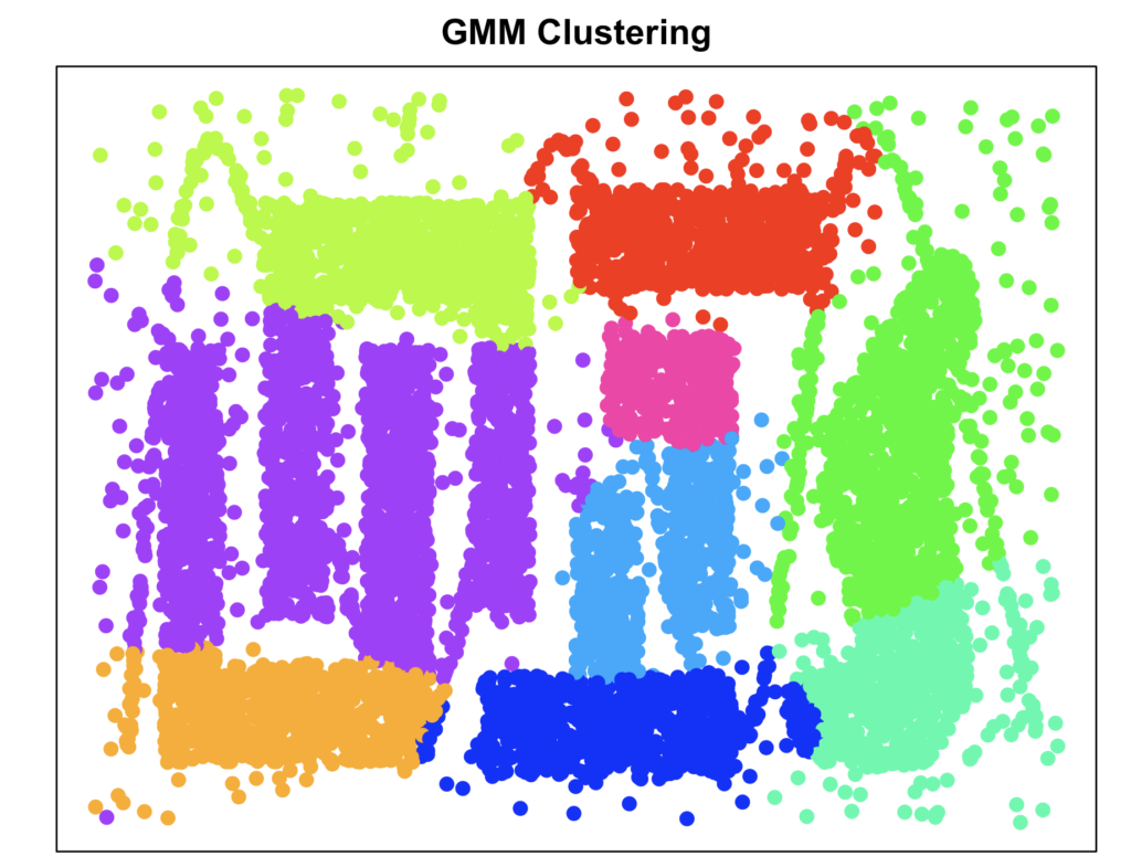
Gaussian Mixture Models seem to not capture the intricacies of this dataset. This was to be expected since the data was not generated by various bivariate gaussian normal distributions.
Ordering Points To Identify Clustering Structure (OPTICS)
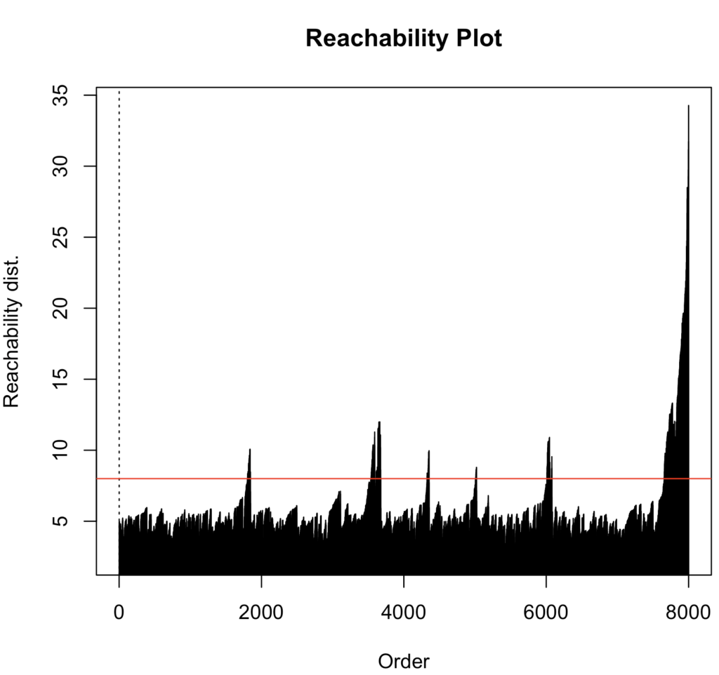
OPTICS is a density-based clustering algorithm that identifies clusters by analyzing the reachability distance between data points. It does not require specifying the number of clusters in advance and produces a reachability plot. This plot reflects the reachability distances between points. Valleys reflect points close together (dense clusters), and peaks indicate transitions between clusters.
Advantages
- Can identify nested cluster structures due to hierarchical nature
- Epsilon parameter does not have to be estimated (in DBSCAN points are categorised in the same cluster if they are within a radius of epsilon from each other),
- Performs well on varying cluster densities since epsilon is not fixed for all clusters (Data Mining, Text Mining, Kunstliche Intelligenz, 2020)
- Can identify noise points
Disadvantages
- Extracting clusters from reachability plot can be complicated, the K-xi method can be used to formalise this (Charlon, z.d.) but that parameter also needs to be tuned
- Reachability plot becomes harder to interpret with larger datasets
- Specifying minPts (minimal number of points a cluster should consist of) is somewhat arbitrary.
I chose minPts to be 10, somewhat arbitrarily but given the number of datapoints this seemed plausible. For the reachability plot I eye-balled the optimal epsilon parameter, i.e., a reachability distance that is above all the values but below all the peaks. I derived the clusters by extracting them with DBSCAN (epsilon = 8)
					cluster_optics_rp <- optics(data, minPts = 10)
plot(cluster_optics_rp)
abline(h = 8, col = "red")
cluster_optics <- extractDBSCAN(cluster_optics_rp, eps_cl = 8)$cluster
noise_index_optics <- which(cluster_optics == 0)
plot_clusters(data, cluster_optics, "OPTICS Clustering")
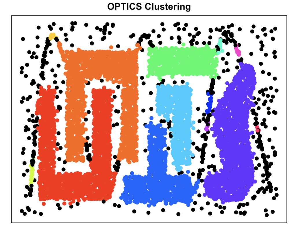
As you can see, OPTICS did a great job in recovering the clusters, due to the density based approach, OPTICS handles non-conventional cluster shapes very well.
Hierarchical Density-Based Spatial Clustering of Applications with Noise (HDBSCAN)
HDBSCAN is a density-based clustering algorithm that extends DBSCAN by building a hierarchical tree of clusters based on varying density levels. It does not require specifying the number of clusters in advance and automatically determines clusters by stability analysis, identifying meaningful groupings while filtering out noise. Unlike traditional hierarchical clustering, HDBSCAN produces a condensed cluster tree, which can be used to explore cluster structures at different density thresholds.
Advantages
- All the advantages of OPTICS and most other clustering methods.
- Does determine the most optimal number of clusters itself. No need to specify K-xi parameter for cluster extraction.
Disadvantages
- Specifying minPts (minimal number of points a cluster should consist of) is somewhat arbitrary.
					hdbscan <- hdbscan(data, minPts = 10)
plot(hdbscan)
cluster_hdbscan = hdbscan$cluster
noise_index_hdbscan <- which(cluster_hdbscan == 0)
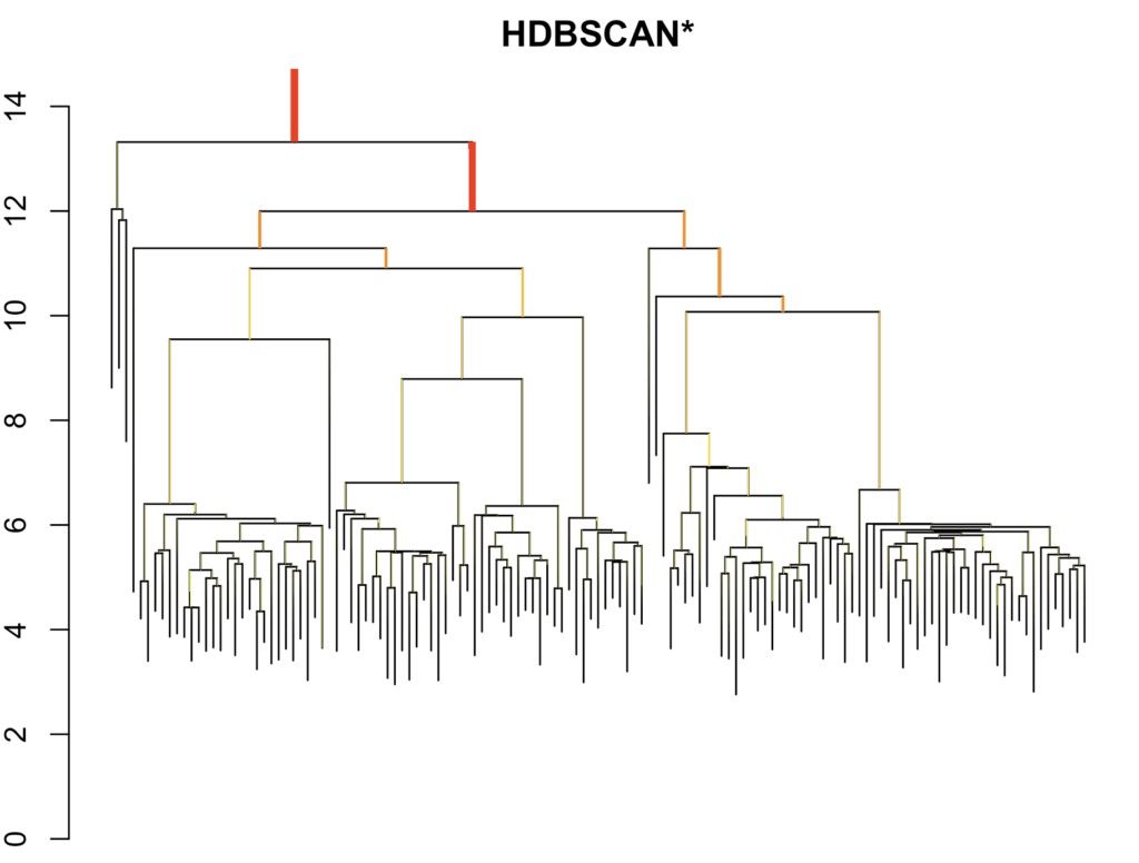
plot_clusters(data, cluster_hdbscan, "HDBSCAN Clustering")
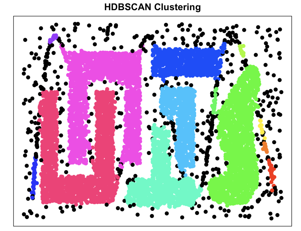
As you can see, HDBSCAN did an excellent job, comparable with OPTICS. However, here we did not have to specify the number of clusters ourselves based on eye-balling or the K-xi parameter, which is a huge advantage.
Conclusion
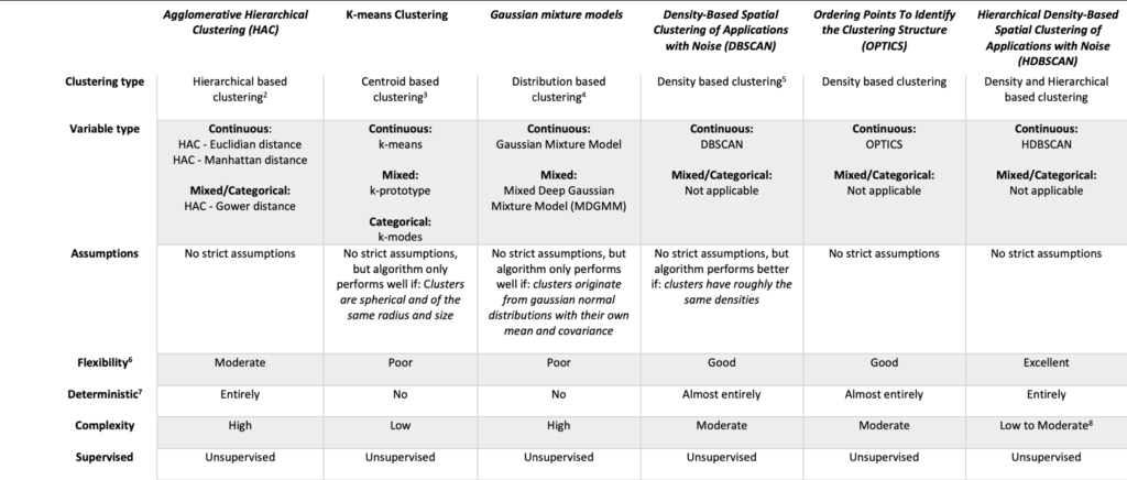
For those who haven’t tuned out yet 😉, I hope this provided insight into advanced clustering algorithms and highlighted that the most popular methods often perform well only under ideal conditions—conditions that rarely exist in real-world data. Fortunately, there are powerful alternatives with simple implementations that can handle more complex structures. Below I added a more formal comparison on various other metrics. Thanks for reading!
References
Tamara Broderick. (2021, 17 mei). MIT: Machine Learning 6.036, Lecture 13: Clustering (Fall 2020) [Video]. YouTube. https://www.youtube.com/watch?v=BaZWcSq3IuI
Data Mining, Text Mining, Künstliche Intelligenz. (2022, 2 June). CLUD8: Cluster Extraction from the OPTICS Cluster Order [Video]. YouTube. https://www.youtube.com/watch?v=VziKnZSffRc
Charlon, T. & University of Geneva. (z.d.). OPTICS K-XI Density-Based Clustering. University Of Geneva. https://cran.r-project.org/web/packages/opticskxi/vignettes/opticskxi.pdf
Rukmi, A. M., & Iqbal, I. M. (2017). Using k-means++ algorithm for researchers clustering. AIP Conference Proceedings. https://doi.org/10.1063/1.4994455
Syakur, M. A., Khotimah, B. K., Rochman, E. M. S., & Satoto, B. D. (2018). Integration K-Means Clustering Method and Elbow Method For Identification of The Best Customer Profile Cluster. IOP Conference Series: Materials Science And Engineering, 336, 012017. https://doi.org/10.1088/1757-899x/336/1/012017
Leave a Reply